SenTrEv (Sentence Transformers Evaluator) is a python package that is aimed at running simple evaluation tests to help you choose the best embedding model for Retrieval Augmented Generation (RAG) with your text-based documents.
SenTrEv works with:
- Dense text encoders/embedders loaded through the class
SentenceTransformerin the python packagesentence_transformers - Sparse text encoders/embedders loaded through the class
SparseTextEmbeddingsin the python packagefastembed - PDF, PPTX, DOCX, HTML, CSV and XML documents (single and multiple uploads supported)
- Qdrant vector databases (both local and on cloud)
You can install the package using pip (easier but no customization):
python3 -m pip install sentrevOr you can build it from the source code (more difficult but customizable):
# clone the repo
git clone /~https://github.com/AstraBert/SenTrEv.git
# access the repo
cd SenTrEv
# build the package
python3 -m build
# install the package locally with editability settings
python3 -m pip install -e .SenTrEv applies a very simple evaluation workflow:
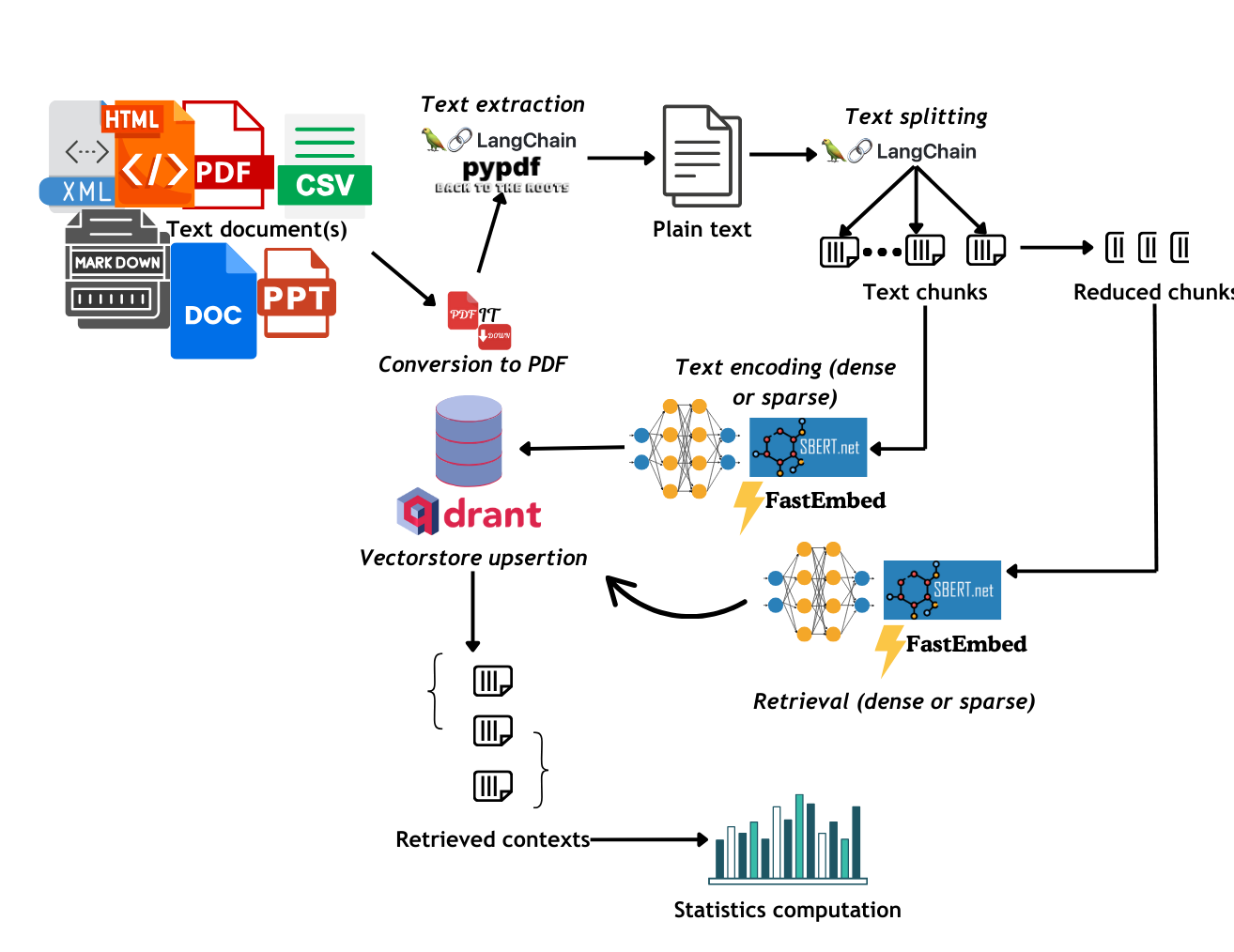
- After the PDF text extraction and chunking phase, the chunks are reduced according to a (optionally) user-defined percentage (default is 25%), which is randomly extracted at any point of each chunk.
- The reduced chunks are mapped to their original ones in a dictionary
- Each model encodes the original chunks and uploads the vectors to the Qdrant vector storage
- The reduced chunks are then used as queries for dense retrieval
- Starting from retrieval results, accuracy, time and carbon emissions statistics are calculated and plotted.
See the figure below for a visualization of the workflow
The metrics used to evaluate performance were:
-
Success rate: defined as the number retrieval operation in which the correct context was retrieved ranking top among all the retrieved contexts, out of the total retrieval operations:
$SR = \frac{Ncorrect}{Ntot}$ (eq.1) -
Mean Reciprocal Ranking (MRR): MRR defines how high in ranking the correct context is placed among the retrieved results. MRR@10 was used, meaning that for each retrieval operation 10 items were returned and an evaluation was carried out for the ranking of the correct context, which was then normalized between 0 and 1 (already implemented in SenTrEv). An MRR of 1 means that the correct context was ranked first, whereas an MRR of 0 means that it wasn't retrieved. MRR is calculated with the following general equation:
$MRR = \frac{ranking + Nretrieved - 1}{Nretrieved}$ (eq.2)When the correct context is not retrieved, MRR is automatically set to 0. MRR is calculated for each retrieval operation, then the average and standard deviation are calculated and reported.
-
Precision: number of relevant documents out of the total number of retrieved documents. The relevance of the document is evaluated based on the "page" metadata entry: it the retrieved document comes from the same page of the query, the document is considered relevant.
-
Non-Relevant Ratio: number of non-relevant documents out of the total number of retrieved documents. Relevance is evaluated as explained in the previous point.
-
Time performance: for each retrieval operation the time performance in seconds is calculated: the average and standard deviation are then reported.
-
Carbon emissions: Carbon emissions are calculated in gCO2eq (grams of CO2 equivalent) through the Python library
codecarbonand were evaluated for the Austrian region. They are reported for the global computational load of all the retrieval operations.
You can easily run Qdrant locally with Docker:
docker pull qdrant/qdrant:latest
docker run -p 6333:6333 -p 6334:6334 qdrant/qdrant:latest
Now your vector database is listening at http://localhost:6333
Let's say we have several text-based files (~/data/attention_is_all_you_need.pdf, ~/data/generative_adversarial_nets.pdf, ~/data/narration.docx, ~/data/call-to-action.html, ~/data/test.xml) and we want to test dense retrieval with three different encoders (sentence-transformers/all-MiniLM-L6-v2 , sentence-transformers/sentence-t5-base, sentence-transformers/all-mpnet-base-v2) and sparse retrieval with three others (Qdrant/bm25, prithivida/Splade_PP_en_v1, Qdrant/bm42-all-minilm-l6-v2-attentions)
We can do it with this very simple code:
from sentence_transformers import SentenceTransformer
from qdrant_client import QdrantClient
from fastembed import SparseTextEmbedding
from sentrev.evaluator import evaluate_dense_retrieval, evaluate_sparse_retrieval
import os

# Load all the dense embedding models
encoder3 = SentenceTransformer('sentence-transformers/all-mpnet-base-v2', device="cuda")
encoder5 = SentenceTransformer('sentence-transformers/all-MiniLM-L12-v2', device="cuda")
encoder6 = SentenceTransformer('sentence-transformers/LaBSE', device="cuda")

# Create a list of the dense encoders
encoders = [encoder3, encoder5, encoder6]

# Create a dictionary that maps each encoder to its name
encoder_to_names = {
    encoder3: 'all-mpnet-base-v2',
    encoder5: 'all-MiniLM-L12-v2',
    encoder6: 'LaBSE',
}

# Collect data
pdfs = ["~/data/attention_is_all_you_need.pdf", "~/data/generative_adversarial_nets.pdf", "~/data/narration.docx", "~/data/call-to-action.html", "~/data/test.xml"]

# Create Qdrant client
client = QdrantClient("http://localhost:6333")

# Set distances
distances = ["cosine", "dot", "euclid", "manhattan"]

# Loop through different chunking_size, text_percentage and distance options
for chunking_size in range(500,2000,500):
    for text_percentage in range(40, 100, 20):
        perc = text_percentage/100
        for distance in distances:
            os.makedirs(f"dense_eval/{chunking_size}_{text_percentage}_{distance}/")
            csv_path = f"dense_eval/{chunking_size}_{text_percentage}_{distance}/stats.csv"
            evaluate_dense_retrieval(pdfs, encoders, encoder_to_names, client, csv_path, chunking_size, text_percentage=perc, distance=distance, mrr=10, carbon_tracking="AUT", plot=True)

# Load all the sparse embedding models
sparse_encoder1 = SparseTextEmbedding("Qdrant/bm25")
sparse_encoder2 = SparseTextEmbedding("prithivida/Splade_PP_en_v1")
sparse_encoder3 = SparseTextEmbedding("Qdrant/bm42-all-minilm-l6-v2-attentions")

# Create a list of the sparse encoders
sparse_encoders = [sparse_encoder1, sparse_encoder2, sparse_encoder3]

# Create a dictionary that maps each sparse encoder to its name
sparse_encoder_to_names = {
    sparse_encoder1: 'BM25',
    sparse_encoder2: 'Splade',
    sparse_encoder3: 'BM42',
}

# Loop through different chunking_size, text_percentage and distance options
for chunking_size in range(500,2000,500):
    for text_percentage in range(40, 100, 20):
        perc = text_percentage/100
        for distance in distances:
            os.makedirs(f"sparse_eval/{chunking_size}_{text_percentage}_{distance}/")
            csv_path = f"sparse_eval/{chunking_size}_{text_percentage}_{distance}/stats.csv"
            evaluate_sparse_retrieval(pdfs, sparse_encoders, sparse_encoder_to_names, client, csv_path, chunking_size, text_percentage=perc, distance=distance, mrr=10, carbon_tracking="AUT", plot=True)
You can play around with the chunking of your PDF by setting the chunking_size argument or with the percentage of text used to test retrieval by setting text_percentage or with the distance metric used for retrieval by setting the distance argument or with the mrr settings by tuning the number of retrieved items (in this case 10); you can also pass plot=True if you want plots for the evaluation: plots will be saved under the same folder of the CSV file; if you want to turn on carbon emissions tracking, you can use the carbon_tracking option followed by the three-letters ISO code of the State you are in.
You can also exploit Qdrant on-cloud database solutions (more about it here). You just need your Qdrant cluster URL and the API key to access it:
from qdrant_client import QdrantClient

client = QdrantClient(url="YOUR-QDRANT-URL", api_key="YOUR-API-KEY")
This is the only change you have to make to the code provided in the example before.
You can use SenTrEv also to chunk, vectorize and upload your PDFs to a Qdrant database.
from sentrev.evaluator import upload_pdfs

encoder = SentenceTransformer('sentence-transformers/all-MiniLM-L6-v2')
pdfs = ['~/pdfs/instructions.pdf', '~/pdfs/history.pdf', '~/pdfs/info.pdf']
client = QdrantClient("http://localhost:6333")

upload_pdfs(pdfs=pdfs, encoder=encoder, client=client)
As for before, you can also play around with the chunking_size argument (default is 1000) and with the distance argument (default is cosine).
You can also upload PDFs to a sparse collection:
from sentrev.evaluator import upload_pdfs_sparse
from fastembed import SparseTextEmbedding

sparse_encoder1 = SparseTextEmbedding("Qdrant/bm25")
pdfs = ['~/pdfs/instructions.pdf', '~/pdfs/history.pdf', '~/pdfs/info.pdf']
client = QdrantClient("http://localhost:6333")

upload_pdfs_sparse(pdfs=pdfs, encoder=None, sparse_encoder=, client=client)
You can also load other documents that are not PDFs, upon conversion to PDFs:
from sentrev.evaluator import to_pdf

files = ['~/pdfs/instructions.md', '~/pdfs/history.docx', '~/pdfs/info.html', '~/pdfs/info.xml']
pdfs = to_pdf(files)You can also search already-existent collections in a Qdrant database with SenTrEv:
from sentrev.utils import NeuralSearcher

encoder = SentenceTransformer('sentence-transformers/all-MiniLM-L6-v2')
collection_name = 'customer_help'
client = QdrantClient("http://localhost:6333")

searcher = NeuralSearcher(client=client, model=encoder, collection_name=collection_name)
res = searcher.search("Is it possible to pay online with my credit card?", limit=5)
If your collection is of a sparse type, you can use this code:
from sentrev.utils import NeuralSearcher
from fastembed import SparseTextEmbedding

sparse_encoder1 = SparseTextEmbedding("Qdrant/bm25")

collection_name = 'customer_help'
client = QdrantClient("http://localhost:6333")

searcher = NeuralSearcher(client=client, model=None, collection_name=collection_name)
res = searcher.search_sparse("Is it possible to pay online with my credit card?", sparse_encoder1, limit=5)
The results will be returned as a list of payloads (the metadata you uploaded to the Qdrant collection along with the vector points).
If you used SenTrEv upload_pdfs/upload_pdfs_sparse function, you should be able to access the results in this way:
text = res[0]["text"]
source = res[0]["source"]
page = res[0]["page"]You can refer to the test case reported here
Find a reference for all the functions and classes here
Contributions are always welcome!
Find contribution guidelines at CONTRIBUTING.md
This project is open-source and is provided under an MIT License.
If you used SenTrEv, please cite:
Bertelli, A. C. (2024). SenTrEv - Simple evaluation for dense and sparse retrieval on your documents (v1.0.0). Zenodo. https://doi.org/10.5281/zenodo.14583071
If you found it useful, please consider funding it .

