In the previous section, you learned about the simplest neural network model - one-layered perceptron, a linear two-class classification model.
In this section we will extend this model into a more flexible framework, allowing us to:
- perform multi-class classification in addition to two-class
- solve regression problems in addition to classification
- separate classes that are not linearly separable
We will also develop our own modular framework in Python that will allow us to construct different neural network architectures.
Let's start with formalizing the Machine Learning problem. Suppose we have a training dataset X with labels Y, and we need to build a model f that will make most accurate predictions. The quality of predictions is measured by Loss function ℒ. The following loss functions are often used:
- For regression problem, when we need to predict a number, we can use absolute error ∑i|f(x(i))-y(i)|, or squared error ∑i(f(x(i))-y(i))2
- For classification, we use 0-1 loss (which is essentially the same as accuracy of the model), or logistic loss.
For one-level perceptron, function f was defined as a linear function f(x)=wx+b (here w is the weight matrix, x is the vector of input features, and b is bias vector). For different neural network architectures, this function can take more complex form.
In the case of classification, it is often desirable to get probabilities of corresponding classes as network output. To convert arbitrary numbers to probabilities (eg. to normalize the output), we often use softmax function σ, and the function f becomes f(x)=σ(wx+b)
In the definition of f above, w and b are called parameters θ=⟨w,b⟩. Given the dataset ⟨X,Y⟩, we can compute an overall error on the whole dataset as a function of parameters θ.
✅ The goal of neural network training is to minimize the error by varying parameters θ
There is a well-known method of function optimization called gradient descent. The idea is that we can compute a derivative (in multi-dimensional case call gradient) of loss function with respect to parameters, and vary parameters in such a way that the error would decrease. This can be formalized as follows:
- Initialize parameters by some random values w(0), b(0)
- Repeat the following step many times:
- w(i+1) = w(i)-η∂ℒ/∂w
- b(i+1) = b(i)-η∂ℒ/∂b
During training, the optimization steps are supposed to be calculated considering the whole dataset (remember that loss is calculated as a sum through all training samples). However, in real life we take small portions of the dataset called minibatches, and calculate gradients based on a subset of data. Because subset is taken randomly each time, such method is called stochastic gradient descent (SGD).
One-layer network, as we have seen above, is capable of classifying linearly separable classes. To build a richer model, we can combine several layers of the network. Mathematically it would mean that the function f would have a more complex form, and will be computed in several steps:
- z1=w1x+b1
- z2=w2α(z1)+b2
- f = σ(z2)
Here, α is a non-linear activation function, σ is a softmax function, and parameters θ=<w1,b1,w2,b2>.
The gradient descent algorithm would remain the same, but it would be more difficult to calculate gradients. Given the chain differentiation rule, we can calculate derivatives as:
- ∂ℒ/∂w2 = (∂ℒ/∂σ)(∂σ/∂z2)(∂z2/∂w2)
- ∂ℒ/∂w1 = (∂ℒ/∂σ)(∂σ/∂z2)(∂z2/∂α)(∂α/∂z1)(∂z1/∂w1)
✅ The chain differentiation rule is used to calculate derivatives of the loss function with respect to parameters.
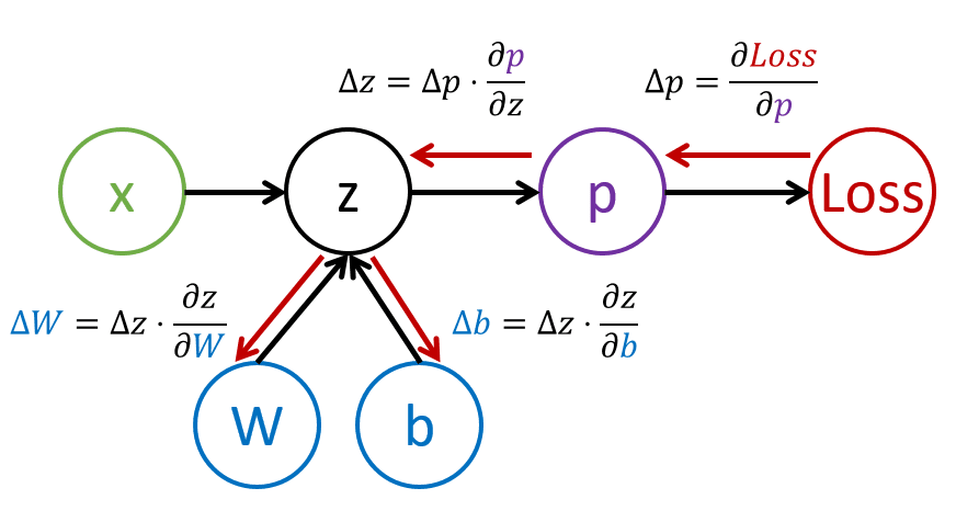
Note that the left-most part of all those expressions is the same, and thus we can effectively calculate derivatives starting from the loss function and going "backwards" through the computational graph. Thus the method of training a multi-layered perceptron is called backpropagation, or 'backprop'.
TODO: image citation
✅ We will cover backprop in much more detail in our notebook example.
In this lesson, we have built our own neural network library, and we have used it for a simple two-dimensional classification task.
In the accompanying notebook, you will implement your own framework for building and training multi-layered perceptrons. You will be able to see in detail how modern neural networks operate.
Proceed to the OwnFramework notebook and work through it.
Backpropagation is a common algorithm used in AI and ML, worth studying in more detail
In this lab, you are asked to use the framework you constructed in this lesson to solve MNIST handwritten digit classification.
